In this paper, we consider the following isentropic compressible Navier-Stokes equations in the one-dimensional region Q: For any T>0, the initial value satisfies the constraint condition: where P=P(C,T), u=u(T) and pu Represent density, speed, and momentum, respectively. The pressure is P(P)=Ap7, A> 0, 7>1, and the viscosity coefficient p is a normal number. For the sake of simplicity, we take A = 1. Area 0 takes a unit interval or a period of period 1. The corresponding boundary condition is: Period Boundary Condition: p, u About Period 1, GR1. (1.4) 2 English citation format: For the initial boundary value problems (1.1)-(1.4), we are interested in the global entropy weak solution (see Definition 2.1) dynamic behavior of the vacuum state, mainly based on the following reasons: As we all know, the initial density is consistent The one-dimensional compressible Navier-Stokes equations have global strong solutions (smooth or piecewise smooth) away from the vacuum. For the high-dimensional case, the strong solution (classical solution) exists when the initial state is close to the non-vacuum equilibrium state, but there is only an adequate large pressure parameter for an arbitrarily large initial value (possibly containing a vacuum) and limited energy. 7 The global weak solution. Therefore, examining the regularity, uniqueness and qualitative behavior of weak solutions are still the focus of our research. The main difficulty here is that there may be a vacuum. Indeed, the smooth solution of a compressible Navier-Stokes equation with vacuum will blow up in a limited time. Even if the initial state contains a little vacuum, the Stokes approximate system smooth solution on the bounded area still has the blasting phenomenon.
Therefore, in order to examine the regularity, uniqueness, and qualitative behavior of weak solutions, it is natural to understand the dynamic behavior of vacuum states. An interesting question between them is if there is no vacuum at first, then if there will be vacuum formation at a later time, we already know the weak solution to the one-dimensional or high-dimensional spherical symmetry compressible Navier-Stokes equation. If there is no vacuum at the beginning, then There will be no vacuum for a limited period of time. In fact, the main theorem in Chinese shows that for any open set ECR and ugly>0, if G,m) is a weak solution of equations (1.1) and (1.2) and then for any te. It also shows that due to mass conservation, the fluid The algebraic rate of (1+t) will expand outwards, the fluid density decays to zero, and the initial vacuum structure of the weak solution will remain. A key fact here is that the constant viscosity coefficient is non-degenerate near the vacuum state. We can obtain a priori estimate of the velocity so that the proton orbit can be defined everywhere and the movement of the vacuum boundary and the upper and lower bounds of the density around the vacuum can be tracked.
In this paper we will show that for any entropy weak solution, if there is no vacuum in the initial state, then the density function is continuous and positive everywhere with respect to time and space variables. Furthermore, we also proved the existence of the global entropy weak solution of a vacuum state containing one or a finite number of intermittent connections. The vacuum region was compressed to a point at algebraic rate and disappeared within a limited time. This phenomenon is consistent with the conclusion that the viscous dependent density compressible fluid in the medium.
Main results We have given the definition of the entropy weak solutions of the initial boundary value problems (1.1)-(1.4) as follows: Definition 2.1 Satisfaction (p, the entropy weak solutions of the initial boundary value problems (1.1)-(1.4), if satisfied and the One of the main results is to reveal that any global entropy weak solution of the one-dimensional compressible Navier-Stokes equation does not produce a vacuum after the initial state without vacuum.
(Vacuum is not formed) Assume that 7>1, pGW1, (1) ((4) and uG ((4). For any arbitrary G, (p, u) is the weak initial entropy (1.1)-(1.4) in the meaning of definition 2.1. Solution B. I (p, u) is strong and satisfies (1) where the entropy estimate (2.3) implies that the density is continuous with respect to time and space variables. In fact, for 7 >1 and IGQ, we can Prove that PGC(xQ) can be obtained.
(2) Theorem 2.1 implies that as long as there is no vacuum at first, the vacuum state of any global entropy weak solution of one-dimensional compressible Navier-Stokes equation must not be generated. It is a special case of the conclusion that the vacuum state of Hoff and Smoller-dimensional compressive fluids will not form.
On the one hand, Theorem 2.1 implies that as long as there is no vacuum at all in the initial state, the one-dimensional compressible Navier-Stokes equation does not produce a vacuum solution for the global entropy weak solution. On the other hand, it is proved that for a compressible Navier-Stokes equation with a viscosity coefficient >0, any finite vacuum will disappear within a limited time. A natural question is whether the vacuum state of the constant viscosity coefficient equations (1.1)-(1.2) disappears within a limited time. If a finite vacuum exists initially, how the dynamic behavior of the vacuum is similar to ours at Qo=(, ) C (0,1) Consider the dynamic behavior of a vacuum with intermittent connections: In order to discuss the dynamic behavior with such a vacuum, we introduce the following definition of "stepwise entropy weak solution".
We call (p, u) the piecewise entropy weak solutions of the initial boundary value problems (1.1)-(1.4) and the initial value conditions (2.7), if it satisfies equations (1.1) and (1.2) to hold in the distributed sense. That is, for any GX), the 0G(1)X solution can be understood as two entropy weak solutions on the old one.
(Vacuum compressible) If 7>1 and initial conditions (2.7) are established. Then there are global piecewise entropy weak solutions in the meaning of definition 2.2 in the initial boundary value problems (1.1)-(1.4). In particular, this piecewise entropy weak solution contains a vacuum state that is compressible and disappears within a limited time. If M(t) =: mesp(C, r) = 0 is the total measure of vacuum, then there is> (2) before the vacuum disappears within a limited time, the fluid propagates along the proton orbit at the boundary of the vacuum. We can use the regions separated by the proton orbits to represent the total measure of the vacuum area. In fact, let a(T) and =(t) define the two proton orbits as follows: then the global weak solution (p, u) of the initial-boundary value problem (1.1)-(1.4) satisfies the fluid along the proton orbit at the vacuum boundary. Propagation, the measurement of the vacuum area can prove (see section 3.2 below) there is a finite time T2> 0, so that when t4T2, there is M(t)40. Proof of the main result 3.1 The vacuum is not formed in this part, we list some basic The fact that it can be proved that the vacuum of the global entropy weak solution to the initial-boundary value problem (1.1)-(1.4) satisfying the non-vacuum initial value will not be formed.
Lemma 3.1.1 If 7>1, T>0, and (p, are the entropy weak solutions of the initial-boundary value problems (1.1)-(1.4), then there is only an initial value constant c>0, so further that we It has been proved that we consider the initial boundary value problem (1.1)-(1.4) in a bounded region that satisfies Dirichlet or periodic conditions. Any 7> 1, and choosing s = is obtained by the Sobolev embedding theorem and (2.3) Can be introduced (3.1).
Therefore, due to the proposition 5.1 in Chinese, we can obtain the lower bound of the density for the global entropy weak solution (p, u) of the initial boundary value problem (1.1)-(1.4) under Dirichlet and periodic boundary conditions.
Lemma 3.1.2 For the global entropy weak solution (p, u) of the arbitrary initial boundary value problem (1.1)-(1.4), the existence time T proves the reasoning method we use. First of all, from mass conservation to unequal entropy > 0, free boundary value problems (3.27)-(3.30) can be decomposed into the following two free boundary value problems and we only need to deal with the problem (I). The problem can be treated similarly.
NOTE 3.1 Equation (I) and boundary conditions imply that the density declines along the free boundary as follows, and the following Lemma 3.2.1 provides a consistent estimate of the derivative of the density function. The proof of Lemma 3.2.1 is similar to Lemma 3.1.1. Lemma 3.2.1 Any y>1, (P,u) is the problem (I) Smooth solution, for any tG, then C>0 is the time Irrelevant constants.
It is evident that we only need to prove (3.35), which is similar to the proof of Lemma 3.2. In fact, in the following boundary bars through complex calculations, we can obtain that we here apply Note 3.1. (p, w is the free boundary value problem (I) entropy weak solution. Then for any y> 1, there is a constant constant AGbookmark15 where When 1 proves first, prove the first inequality of (3.37).bookmark17 applies the energy function bookmark18 to the free boundary value problem (I) to deal with i3.T.T) Therefore, substitute the estimates of l2 and I3 into (3.40), Any Y> The following discussion of Y points: because! = U(p(T), T), with respect to T-integrals, H(t) can be derived from ten to ten times where s is 1 (one ten applies conservation of mass, Holder inequality and (3.46), available p=d D 0, making this part of the interface with vacuum interrupted = a(T) and (t) We need to study the dynamic behavior before the vacuum disappears, the key lemmas are given below.
1. Assume that the vacuum boundary C=a(T) and C= proof are similar to the lemma 3.2.2, for the problem weak solution (p,), the wide T can be obtained where C>0 is a time-independent constant.
A function b similar to (3.39) was introduced (discussed below for the 7-point situation: because !=a(b(T),T), there are ten s for T-integrals. So we therefore have (3.55) and (3.56) are available, so any Y>1, from (3.57) and (3.53), is available, in fact, for the problem (I) in the region ((0,a(T)U(b (T), 1)) The entropy weak solution of x (p, as can be immediately derived from (3.37) (3.50). Lemma 3.2.3 is proven. Mouth 1, (p, is the initial boundary value problem (3.27) If any of (3.31) contains a piecewise entropy weak solution of intermittently connected vacuum states, then this part of the vacuum can be compressed to a non-vacuum point within a limited time, ie, if M(t):=mesp(x, t) = 0, then there is time 13> is> Ti> 0, so here = (a(T), b(T)). The measure of vacuum is easy to prove, in Euclid coordinates (0, a(T) )) The solution of x and (6(t),1)x (p, which can be transformed into the free boundary value problem (I) and the solution in Lagrange coordinates (eight sentences.) is derived from Lemma 3.2.3 so that there is a time T2 >Ti>0, making us assert existence Between To > 0, so that when i > To, p is strictly greater than zero. In fact, if p 0 makes a continuous connection, and it cannot directly determine the vacuum of the vacuum interface when i is normal, we can The total pressure dissipation in the presence of a vacuum is used to prove that (3.64)-(3.66) results are similar to (3.60) and that of Lemma 3.2.4.
æˆ, + +) = p(bci), when i>T2, it can be deduced that any piecewise entropy weak solution (p, M) becomes a weak entropy solution.
The proof of Theorem 2.2 uses Section 3.2 to obtain a priori estimate. It can be proved that the initial density satisfies the global existence of piecewise entropy weak solutions for the initial boundary value problem (3.27)-(3.30) in (3.31). Divided in two steps to prove Theorem 2.2: Step 1 is the same for tGxx and holds true. In addition, it is easy to introduce the second step from Lemma 3.2.3. In order to extend (p, U) into a global solution, we consider the initial (p, U) (T2) problems (3.27)-(3.29). The recording density and speed at both ends of the ==a(T2)=b(T2) limit are for t>T2, we deal with two cases, +, T2), we can push here the normal number determined by p>0 from the front . Therefore, for any t>T2, similar to the problem we can get the initial boundary value = true. Applying the initial boundary value problem (3.27)-(3.29) similar to the one in the lemma 4.1-4.5, there is a global piecewise entropy weak solution that contains the defined curve C=C(1) along this curve Rankine- The Hugoniot condition holds: Here the piecewise entropy weak solution. Theorem 2.2 proves.
Acknowledgments The authors sincerely thank the reviewers for their valuable suggestions.
This producing line is suit for coils in different specification, through uncoiler, flattening, slitter, cutting, finally form a plate in needed length.
This producing line is suit for coils in different specification, through uncoiler, flattening, cutting, finally form a plate in needed length.
This series of producing lines apply to different model of coils. Through uncoil, checking level and cutting, this producing line offer the tidy sheet for special length and width
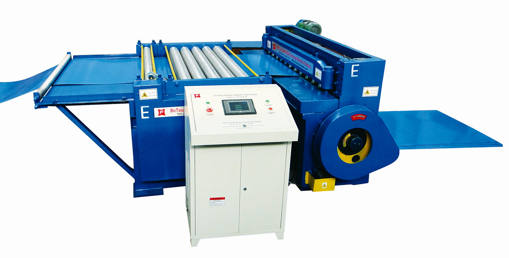
Uncoiling Flatting Cutting
Uncoiling Flatting Cutting,Uncoiler-Slitting-Recoiling Machine, Uncoiler Machine, Recoiling Machine
Botou Xianfa Roll Forming Machine Factory , https://www.rollforming.nl